Methodological Issues in Event-Related Brain Potential and Magnetic Field Studies

Walton T. Roth, Judith M. Ford, Adolf Pfefferbaum, and Thomas R. Elbert

Psychiatry in its search for the roots of abnormal thoughts, feelings, and behavior has again turned its attention to the human brain and is trying to apply the methods of the many scientific disciplines that have cast light on normal brain functioning-disciplines such as neuroanatomy and histology, biochemistry and molecular biology, and electrophysiology. This chapter concentrates on ways of maximizing what can be learned from noninvasive electrophysiology, a technique that is singular in its ability to record millisecond-by-millisecond changes in the brain following repeated external or internal events. Although the triggering events are often simple sensory stimuli, the cognitive processes that follow them and leave their trace in fluctuating voltage or magnetic fields can be quite complex. In the last decade competing noninvasive techniques such as positron emission tomography (PET) have challenged the preeminence of electrophysiology, particularly in spatial localization of brain processes. This challenge has stimulated a number of technological and methodological developments in acquiring, analyzing, and presenting brain electrical and magnetic data. But before we review these developments, we remind you of some basic principles and give examples of their relevance to psychiatry (see also A Critical Analysis of Neurochemical Methods for Monitoring Transmitter Dynamics in the Brain, Electrophysiology, and Pharmacology and Physiology of Central Noradrenergic Systems for related discussion).

Nerve cells generate extracellular current flow by fluctuations in the slower changing membrane potentials of dendrites and cell bodies. Postsynaptic potentials cause an outflow of negative (excitatory) or positive (inhibitory) ionic charges into extracellular fluid, which are then pumped back into the cell. This current flow, when summated, results in volume-conducted potentials recorded at the scalp as the electroencephalogram (EEG). Event-related potentials (ERPs) are EEG changes that are time-locked to sensory, motor, or cognitive events. They have provided a way to evaluate brain functioning in mental disorders and the effects of psychoactive drugs. Recent conceptual and technical developments have greatly expanded our capability to understand and document the mechanisms underlying surface recordings. Particular attention has been paid to identifying the location, orientation, and distribution of current dipoles (pairs of opposite charges) that may be the sources of scalp-recorded electrical activity.

Nerve cells also generate intracellular current flow from dendrites to cell body. This flow results in a magnetic field that can be detected at the scalp as a magnetoencephalogram (MEG), even though it is a billionfold less intense than the earth's magnetic field. Event-related magnetic fields (ERFs) can be elicited and time-locked to specific events and are analogous to ERPs. Magnetoencephalograms and ERFs convey different information than EEG and ERPs. This is because voltage fields on the surface of a sphere, which the skull enclosing the brain approximates, are produced equally well by dipoles oriented radially and tangentially with respect to a radius of the sphere. In contrast, 90% of the magnetic field at the skull can be ascribed to tangential dipoles alone. This is a consequence of the geometrical orientation of masses of nerve cells and of magnetic sensors. Fig. 1 illustrates how dipole orientation can be either correlated or random for different gyri and sulci. Parallel dipoles lying tangentially on sulcal walls contribute much more to the MEG than random dipoles or dipoles lying radially along the crowns of gyri.

Why are the methodological issues that this chapter addresses relevant to psychiatrists and psychologists? First, ERPs and ERFs are theoretically relevant because they provide ways of testing theories of abnormal brain functioning that no other methods can offer. For example, unlike ordinary behavioral tests of cognitive processing, ERPs give an index of the processing of task-irrelevant events, distracting stimuli, or events subjects have been told to ignore. The topographic distribution of ERPs and ERFs gives clues as to what parts of the brain are active during a particular cognitive activity. Second, ERPs and to a less extent ERFs have been demonstrated empirically to be relevant. ERP abnormalities have been repeatedly observed in psychiatric disorders, notably in the P300 and P50 components. The P or N signifies positive or negative and the number is the mean peak latency in milliseconds. Thus, the P300 component is a positive potential that occurs approximately 300 msec after a stimulus that is infrequent and in some way relevant. The most venerable and consistent psychiatric ERP finding is that of reduced P300 amplitude in schizophrenics (60), although this is not specific to schizophrenia (see refs. 59 and 22 for reviews). For instance, a longitudinal study demonstrated that lower P300 amplitude at age 15 was predictive of poorer global personality functioning at age 25 (66). Latency at P300 is generally greater in patients with dementia than in normals or in patients with schizophrenia or depression (28, 54). Recently, psychiatric attention has been directed to P50, an ERP component to auditory stimuli whose amplitude is suppressed if the eliciting stimulus is paired with another that precedes it by one-half second. Schizophrenics show less P50 suppression than controls (25) as indicated by smaller amplitude ratios (P50 to the second stimulus of a pair divided by P50 to the first), although again this finding is not limited to schizophrenia (4).

Abnormalities of ERPs in psychiatric patients can be interpreted in light of a considerable amount of knowledge that has accumulated about the significance of certain ERP components in normal human information processing. For example, P300 is known to reflect the categorization of events, depending jointly on stimulus probability, stimulus significance, and the information value of the event (36). Probably, P300 has multiple, partially asynchronous generators (58). Components occurring 60 to 100 msec after onset of auditory stimuli, including N100, have been shown to reflect selective attention to auditory stimulus channels (42). In contrast, auditory ERPs with latencies less than 10 msec are insensitive to attention effects but give a unique assessment of the intactness of brainstem circuitry (32).

The literature on ERFs in normal subjects is quite extensive although magnetic recording techniques have been available only a relatively short time. Much of that literature has documented the existence of ERF components that parallel those established by invasive and noninvasive ERP recording. However, to date, most clinical MEG studies have been done in neurological rather than psychiatric patients, although that is likely to change in the near future. Reite et al. (57) recorded ERFs in six medicated, paranoid schizophrenic patients and six normal controls. The M100 component (analogous to the N100 of the ERP) showed less interhemispheric asymmetry in schizophrenics and had different source orientations in the left hemisphere. Tiihonen et al. (68) compared the M100 component in two schizophrenic patients when they were experiencing auditory hallucinations and when they were not. During hallucinations, M100 peaked approximately 20 msec later, an effect similar to that of external masking noise in normals.

We now turn to methodological trends that are transforming ERP and ERF research. Specific topics include data acquisition, signal averaging, ocular artifact, choice of reference electrodes, digital filtering, measuring components including dipole modeling, and statistical and diagnostic considerations.

Older electroencephalographic tube-based amplifiers have been completely replaced with high impedance solid-state amplifiers with electronically controlled amplification and filter settings. In many laboratories, pen-chart recorders have been replaced with electronic data storage and display systems, but paper records are still widely used for visual analysis of diagnostic EEGs and sleep. Laboratory computers are constantly evolving toward faster, cheaper, and more powerful models. New storage media based on tape or magnetic or optical disks permit archiving of data from many subjects in an easily retrievable form. As welcome as these advances have been, they have generated difficult new choices for researchers. Should they buy commercial EEG and ERP hardware and software systems or develop their own? Which commercial systems or routes to laboratory-program development are satisfactory? Commercial systems tend to be limited in flexibility, details of data analysis may be a trade secret (which is unacceptable scientifically), and access to raw data for special analyses may be difficult. Laboratory-developed systems require deciding among manifold hardware and software possibilities, and then allocating many hours to programming. As will be learned from this chapter, methodologically up-to-date ERP analysis requires much more than eye-movement artifact rejection and signal averaging.

Whereas the conventional 10–20 system of Jasper (35) used 19 electrodes with a typical distance of 6 cm between them, some investigators have greatly expanded the electrode arrays in order to record more of the spatial detail present in the EEG. Thus arrays of 124, or even 256 electrodes, which yield interelectrode distances of 2.25 and 1.6 cm, are now being advocated (27) and have been shown to enhance localization. The application of multiple electrodes is a lengthy, labor-intensive process, which requires care in scalp preparation and accuracy in electrode placement. For localization studies relating EEG or MEG data to brain structures visualized by magnetic resonance imaging (MRI), it is important that electrodes be aligned correctly according to skull landmarks, and fiducial markers visible in MRI scans are used. (Vitamin E capsules are easily available and the right size.)

Electrode application entails a potential health risk to both subject and technician if the intactness of the scalp is compromised by procedures to reduce electrical resistance between electrode and scalp or by skin lesions. Acquired immunodeficiency syndrome and hepatitis B can both be transmitted by this route, so it is absolutely essential that proper precautions be taken. Putnam et al. (56) give recommendations for disinfecting reusable electrodes and for protecting the technician.

The recording of the MEG has been made practical by the development of superconducting quantum interference devices (SQUIDs) that are sensitive to minute magnetic fields. The MEG technology is much more expensive than the EEG technology. Not only are the SQUIDs themselves expensive, but they require provision for liquid helium at 4.2°K to cool them, and a recording room shielded with a high-permeability material against magnetic fields and with aluminum against eddy currents. The liquid helium is kept in a vacuum-insulated container called a dewar. Locating magnetic sources requires recording from multiple sites, preferably simultaneously. Otherwise, separate stimulation runs must be made, moving sensors from one location to another between runs. More runs take more recording time and increase the likelihood that the subject's mental state will change, altering the sources. A MEG system with over 30 channels costs approximately $3,000,000, 100 times more than the same number of EEG channels. Because MEG prices reflect the cost of research and development more than construction of the apparatus, the price per unit would drop if more units were sold. In one system, 37 sensors are placed 2.2 cm apart to cover a single hemisphere (12).

An advantage of MEG sensors is that they do not touch the head, so transmission of infectious agents is of less concern. Fixation of head position is critical so that sensors can be aligned according to skull landmarks. Modern SQUID technology allows recording of signals that vary slowly over a minute, undisturbed by electrode drift. A new method for recording even slower or static magnetic fields converts such fields to more rapidly changing fields by having the subject lie on a mechanically driven platform that executes a circular movement of a few centimeters at 0.2 Hz (26). Auditory and visual stimulation cannot be given by conventional earphones or CRT displays because of their magnetic properties. Instead, sounds have to be delivered from outside the testing chamber through hollow tubes and visual stimuli projected through a window in the magnetic shield or delivered fiber optically.

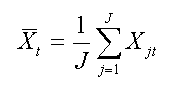
Both ERPs and ERFs benefit greatly from signal averaging to enhance their signal-to-noise ratio (SNR). Data are generally digitized at a fixed rate to fill a data array, and a stimulus or other synchronizing event defines the time epoch of interest within this array. The event is repeated (each repetition is called a trial), and a time-locked signal (ensemble) average is calculated across trials epochs for each time point of the epoch. If Xj(t) is the electrical potential (voltage) or magnetic field strength at some electrode or sensor location at time t and trial j, the signal average is defined as

If Xjt is considered the sum of true signal mt and random noise Njt (background EEG and measurement error), signal averaging improves the SNR. Unbiased estimates of signal power , noise power , and SNR can be calculated as follows (71).

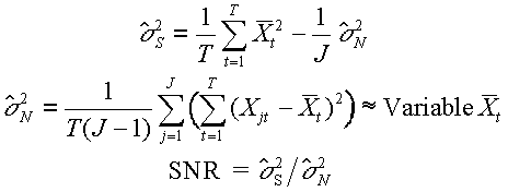
One of the assumptions of signal averaging is that the signal is invariant across trials. This assumption is violated when the amplitude of the ERP component of interest habituates or when its latency varies from trial to trial, as is clearly the case for components related to certain cognitive processes, such as the P300. One way of dealing with component latency variability is to locate the signal on each trial and align the trials on these signals rather than on the eliciting stimulus. Woody (75) proposed an iterative procedure (an adaptive filter) that located the signal on each single trial by moving a template (initially the signal average) by time increments along the trial to find the latency of maximum correlation. A new average was then formed by aligning trials on the identified signal latencies, and the new average was used as a new template. If the SNR is too low, this procedure produces results that simply reflect random noise. Gratton et al. (31) tested the procedure with simulated signals and background EEG noise and demonstrated that iterations (up to three) were important only when the original template had a wavelength on the order of two times longer than the signal.

Roth et al. (56) used this procedure to analyze ERPs elicited from schizophrenics and controls performing an auditory choice reaction time paradigm in order to test whether P300 amplitude reduction in schizophrenics could be attributed to latency variability. They found that individual trial P300 latency was indeed more variable in schizophrenics but that schizophrenic P300 amplitude was still smaller than control amplitude after latency adjustment. To reduce distortions due to noise, Pfefferbaum and Ford (53) modified the procedure by only including trials whose covariance is greater in the part of the epoch where signal is expected than in the part where noise is expected, and whose correlation with the template (initially a half-sine wave) exceeds a set threshold. Using this modified procedure, Ford et al. (23) replicated the Roth et al. (61) finding that schizophrenic P300 remained smaller. Furthermore, schizophrenics had more trials that did not pass the covariance–correlation screen than controls. Trials that did not qualify for latency adjustment had longer reaction times, showing that they were deviant behaviorally as well as electrophysiologically. In addition, Ford et al. calculated for each subject the covariance of P300 signal average across trials with that subject's EEG in single signal epochs and in single nonsignal epochs. The ratio of mean signal covariance to mean noise covariance was significantly smaller in the schizophrenics. Because trials were filtered with a bandpass of 0.5 to 4.4 Hz, noise was EEG activity in the frequency range of P300 rather than higher frequency like a, b, or muscle activity.

Another assumption of signal averaging is that background EEG noise is random noise. This is only an approximation to the truth, as a study of event-related spectral perturbation indicates (41). In normal subjects, auditory tone pips reliably produced momentary increases in spectral power in the 2- to 8-Hz and 10- to 40-Hz bands.

Eye movement and blinks produce electrical potentials and magnetic fields that are often much larger than those deriving from brain sources. The magnetic fields are more restricted to the vicinity of the eye than are the electrical fields and for this reason are less troublesome if unsynchronized with events of experimental interest. Synchronized eye artifact can cause major errors in peak measurement or source localization. Attempts to control this artifact by instructing subjects to fixate their gaze on a point or not to blink are often ineffective, particularly if the subject is psychotic or cognitively impaired. Thus methods for removing eye artifact from the ERP or ERF need to be applied. Many are based on determining the coefficients Ak in the equation

V(k,t) = Ak * EOG(t) + EEG(k,t)

where V(k,t) is the voltage observed in lead k at time t, and EOG(t) and EEG(k,t) are the true EOG and EEG voltage contributions at that time.

Spatial-temporal dipole models of eye movements and blinks make it clear that the same correction cannot be used for both (6). Thus eye-correction procedures should include at a minimum the following steps: (a) Separate blinks from movements on the basis of their temporal properties, (b) calculate separate linear regressions for the propagation of artifacts from each, and (c) correct EEG leads by the amount predicted by the regression coefficients. Gratton et al. (29), whose method has been used by a number of investigators, adds an additional step of subtracting signal averages from individual trials to avoid distortions resulting from ERP effects in both EEG and EOG records. A computerized implementation of this procedure that adjusts for both a vertical and a horizontal EOG channel, has been developed (43). Although certain technical issues in implementing EOG corrections remain unresolved—the proper number and position of EOG electrodes, the error attendant upon assuming a linear relationships between the EOG signal and EEG artifacts, the implications of the presence of EEG artifacts in EOG leads, how to deal with overlapping eye movement and blinks, and instability of individual propagation factors between sessions and even between tasks within a session (19)—the use of such off-line procedures have greatly increased the number of trials available for analysis in clinical studies.

Whereas MEG sensors detect the absolute magnetic field at a given location in space and need no reference in the body, the EEG must be measured as voltage differences between two points on or in the organism. Ideally one point should be close to the biological voltage source under investigation, and the other should be a reference point with constant voltage or at least a voltage not correlated with the source voltage. Traditional references for human ERP have been linked mastoids, linked ears, or the nose; unfortunately none of these is unaffected by brain sources. Special disadvantages of linked ear references include the possibility that shorting can reduce asymmetry if resistance is low, and the possibility that artifactual spatial asymmetry will result if resistances at the two ears are not equal (48). Shorting is not a serious consideration as long as skin-electrode resistance at each ear is greater than 5 kW, because in that case scalp path resistance is reduced less than 5% (44). Resistance at the two ears can be balanced with a potentiometer, or one ear (say A1) can be used as a reference and recorded as a separate channel. Then a linked ear reference for say Cz, a scalp electrode in the 10–20 system, can be created algebraically, (Cz - A1) - (A2 - A1)/2 = Cz - (A1 + A2)/2.

To avoid active reference electrodes on the head, some investigators have turned to noncephalic (e.g., sternovertebral) electrodes (67). Unfortunately these electrodes are liable to pick up heart activity even when adjusted to be at right angles to the main vector of voltage during the cardiac cycle, since cardiac depolarization and repolarization vectors do not maintain a perfectly constant direction over the cycle.

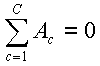
Another solution is to use an average reference. At each time point, an average reference defines zero over C electrodes in a data array A as

A limitation of the average reference is that when electrodes are not densely and equally spaced around the brain, for example, there are none at the bottom of the head (69), the sum in the formula above is generally different from true zero. For example, Desmedt et al. (16) have shown that P14 of the somatosensory evoked response, which is present with a linked ears reference, disappears when a zero reference based on 27 scalp electrodes is applied, becoming surrounded by "ghost" negativities. A linked-ear reference reflects more accurately the medial lemniscal volley that is the presumed basis of P14. In addition, local changes can be mistaken for global changes with a zero reference. These distortions are less likely to affect tangential than radial dipoles.

In conclusion, there is no perfect reference for all cases. As a general principle, a known local source should be referred to an electrode distant from it.

Before measurements are made on ERPs or ERFs, it is useful to apply SNR-enhancing filters that incorporate assumptions about frequency, timing, and spatial distribution of the component of interest. For example, the ERP P300 component may be expected from experiments in the literature to have a frequency lower than 2 Hz (30), to peak in a range of 280 to 400 msec (in a simple auditory choice reaction time task in young adults) and to be maximal at Pz, another electrode in the 10–20 system. Though signal averaging attenuates unsynchronized noise at every frequency as it improves SNR, frequency filters are commonly applied prior to component measurement. These filters are useful whenever the frequency of the noise is different from that of the signal.

Digital frequency filters (11) have the advantage over analog filters of being able to operate without introducing distorting phase shifts into the signal. The most commonly used digital filter has been the moving average or boxcar filter, in which each point of the signal is replaced by an average of that point and a certain number of prior and subsequent points. This is only possible for stored data, because it makes use of future time points to calculate current output. Farwell et al. (20) have shown that a simple moving average filter does not prepare average and single-trial waveforms as well for P300 peak-picking as does a filter designed by an optimizing algorithm. Such an algorithm determines a set of weights that are able to reduce deviations (ripple or ringing) in the passband and stopband of the filter. Optimized filters have less tendency to reduce P300 amplitude or distort shape and, in the case of averages, gave more stable latency measurements. For P300, the authors recommend that the optimum filter have a passband cut-off frequency of 6 Hz, a stopband cut-off frequency of 8 or 8.5 Hz, and use 490/n points, where n is the sampling interval in milliseconds. It should be emphasized that analog filters still have a place in data acquisition prior to digital filtering—a low-pass analog filter with a half-power frequency below but close to half the sampling rate prevents aliasing, and, for P300 recording, a high-pass analog filter with a half-power frequency of less than 0.16 Hz minimizes irrelevant baseline shifts (20).

Current source density maps (also called surface Laplacian or radial current estimate maps) act as spatial filters emphasizing localized components with a high spatial frequency. For this to work well of course, electrodes must be placed with a high spatial frequency. Maps can be made of unaveraged activity such as epileptic spikes or of signal averages. Sensory ERP components show a more localized distribution using this approach than in voltage maps. For example, Nagamine et al. (46) compared voltage and current source density maps on the scalp ERPs obtained by tibial nerve stimulation. The results for a single subject presented in Fig. 2 demonstrate better localization for P40, N50, and P60 for the current source density map. The equation for calculating current source density is I = r(d2V/dx2 + d2V/dy2), where V is the voltage, x and y the surface location on the x–y plane, and r the charge density. In addition, r = k * d2, where d is the distance between electrodes and k is a constant for all electrodes within a subject. The Laplacian operator can give limits for finding equivalent dipoles. It has a physical interpretation—local radial current flow from the brain into the scalp and vice versa—but it is different from dipole modeling (described below) and is free of dipole modeling's ambiguities.

In the Laplacian calculation, surface contours can be generated by a method called spherical spline interpolation, which is based on physical principles for minimizing the deformation energy of a thin sphere constrained to pass through known points (51). This produces a smooth surface running through the data values and filling in between them, even when electrodes are irregularly placed on the scalp. Spherical splines have advantages over plate splines, which are based on deformation of an infinite thin plate. As might be expected from the fact that interpolated values at any point are derived from data from other locations, coherence (a measure of covariation) is inflated by interpolation. Nearest-neighbor interpolations are less smooth and inferior for locating extrema (peaks and troughs must lie on an electrode site) but do not inflate coherence.

Gevins et al. (27) have demonstrated a method of current source density mapping they call finite element model deblurring that they believe is superior to the Laplacian method. Mathematically, it is a less computationally demanding version of dipole modeling known as spatial deconvolution, which assumes that all dipoles are located on a cortical surface. Gevins et al. use the subject's head MRI to provide information about conducting volumes between scalp and cortical surfaces.

A simpler spatial filter, the vector filter (30), has been used for component measurement. Its output is the weighted sum of data points at different electrodes. Conceptually, measuring a component at one lead is the same as applying a vector filter with weight 1 assigned to values at that lead and weight 0 to values at all other leads. Vector filtering assumes that the distribution of the component to be measured is constant despite changes in amplitude or latency. The crux of the procedure is how to specify the weights: using three 10–20 system scalp electrodes, Fz, Cz, and Pz, weights of 0.15 for Fz, -0.53 for Cz, and 0.83 for Pz were found to produce optimal discrimination in an oddball paradigm between rare trials, which contain substantial P300s, and frequent trials, which do not (30). Thus, optimum weights do not necessarily correspond to component distribution, because P300 is larger at Cz than at Fz. Dipole modeling, which is described below, can act as both a spatial and temporal filter.

A component can be defined as electrical or magnetic activity associated with a specific neurological or psychological process, for example, a motor act such as moving one's finger, a sensory process such as the reaction to a light flash, or a cognitive process such as categorizing a stimulus as target or nontarget. In a statistical sense a component explains experimental variance. The details of the experimental method are part of the operational definition of a component. As more experiments are done, theoretical expectations about components develop into generalizations. For example, many experiments in which subjects performed a fixed foreperiod reaction time task have resulted in a parietal–central negative shift prior to the button press. A natural generalization is that the parietal–central shift represents preparation for a motor act. Furthermore, because the source of the recorded data is a physical location within the brain, the ultimate description of a component must include reference to the specific brain structures activated. Some leads or sensors will pick up activity from those structures better than others, particularly when sources are multiple with overlapping influences. In the case of ERPs, the choice of voltage reference influences how electrical activity from a source appears in the EEG recording.

Measurement procedures include peak picking, area measurement, waveform subtraction, principal components analysis, template correlation, and dipole modeling. Peak picking means finding maxima or minima in specified latency ranges and determining peak latency and amplitude with respect to a prestimulus baseline. This is the simplest method of component evaluation, but can be biased when latency ranges are selected after an inspection of the data, and is perhaps unduly restricted in that it considers only peaks among other waveform features. In addition, it is often based on only one point, which may be influenced by noise or overlapping components. With multiple leads, another limitation of peak picking becomes obvious: what appears by shape to be a single component has maxima at different time points in different leads, and it is not clear how best to resolve the discrepancies. Furthermore, the choice of reference electrodes can determine when peaks and troughs appear.

Area measurement is sometimes used when the component is believed to be more rectangular than peaked. Area is measured in a specified latency range, and is thus based on multiple points, but area measurement, like peak picking, can be biased and is influenced by overlapping components.

Waveform subtraction can be used before peak picking or area measurement to reduce the effects of component overlap. For example, consider a paradigm where tones of two pitches are given in an unpredictable sequence and one occurs less frequently and is designated as the target of some task. The ERP to the rare tone can be considered a combination of the sensory effects of the tone and the cognitive effects of the tone being a rare target. By subtracting the ERP to the frequent tones from the ERP to the infrequent tones, the sensory effects are removed leaving behind the cognitive effects. This assumes that the sensory responses to the two tones are identical and that cognitive and sensory effects are additive, an assumption that is not always warranted. For example, frequency-specific temporal recovery of the auditory N100, a noncognitive effect, makes the response of N100 to frequents smaller than the response of N100 to rares.

Principal components analysis (PCA) is another approach to ERP component measurement, which uses the time points on waveforms from different subjects, different electrodes, and different experimental conditions to define components. In statistical terms PCA identifies orthogonal axes of maximal variance in a multidimensional space defined by the variables. Generally these axes are rotated according to the varimax procedure. Less arbitrary than peak picking, PCA makes no assumption about the latency range in which specific components will be found but only that they have a fixed latency across conditions and subjects. It has some ability to separate overlapping components. However, PCA is not completely free from arbitrariness. First, PCA solutions are not unique. Many rotations of the factors are possible. Second, results depend to a certain extent on what experimental conditions are chosen and how many leads are included. Variance from electrodes, subjects, conditions, and correlated noise are all treated the same. Furthermore, each experiment gives slightly different factor structures, and there is no established criterion for deciding whether these differences are significant or not. Thus, it is uncertain how many statistical components to interpret, and how to identify these components with ones previously described.

Template correlation assesses the similarity of a template of the component to the waveform to be evaluated. The template may be based on prior knowledge of the component shape or on signal averages (see the iterative Woody filter procedure described above). The template is usually compared to waveforms at specified intervals over a designated latency range to identify the latency of maximum correlation (or in one variation, maximum covariance). This time point is defined as the peak. The sum of cross products at this time point or the difference between amplitude at this point and a baseline can define amplitude.

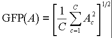
Interpreting latency data under different experimental conditions can be difficult when multiple leads are involved. Latency may vary at different leads and topography may vary under different conditions, implying different components whose latency cannot be compared. To solve these problems, Brandeis et al. (8) spatially generalized the Woody filter procedure using an average reference map, and applying a measure they call global field power (GFP) defined by the following formula for an array A consisting of data from C electrodes:

Further, global dissimilarity (GD) is defined as the root mean square (rms) power of the difference maps calculated by subtracting two normalized GFP maps. The procedure is as follows: (a) Grand averages are used to form template GFP maps, from which component model maps at single latencies near 100, 200, and 400 msec are derived, corresponding to P1, N1, and P3 (see ref. 8 for details). (b) Component model maps are moved in specified latency ranges around the latency of each model's component. The minimum of GD multiplied by sequential dissimilarity (GD between current and previous map: a stability constraint) is calculated, and the minimum of this function (best fit) is defined as the map latency for that component. (c) In an iteration, the average of all normalized maps at their latencies of best fit is used as a new model, and the search window is set around the new mean latency. The results show that components can be identified by topography alone, without respect to amplitude or time. However, this method does not take into account possible overlapping components and would fail if such components influenced topographies. Furthermore, average references for P300, which is widely distributed on the top of the head, may be inferior to a noncephalic reference.

Dipole modeling is a method for reducing data from multilead EEG or multisource MEG by deducing the dipole sources that may have produced them. Although the forward problem (calculating scalp distribution from known dipoles) has a unique solution whose accuracy is limited only by the approximations of skull geometry and conductivities, the inverse problem has multiple mathematically valid solutions as was pointed about by Helmholz more than a century ago (33). The reason is that a single scalp distribution can be produced by different numbers of dipoles in different combinations of locations and orientations. Thus, various constraints on the number of sources allowed and their approximate location must be applied to reach a solution. Sometimes these constraints are so severe as to specify that the source be a single dipole located somewhere in the brain.

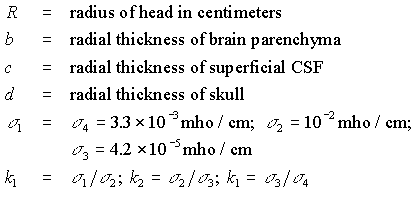
At an abstract level, dipole modeling is like PCA in that an equation U = C * S must be solved where U is an array of k electrodes at t times that represents the linear superimposition of the array S of m sources at t times multiplied by C weighing coefficients at k electrodes for m sources (62). Whereas PCA determines C and S from mathematical constraints, dipole modeling assumes that C depends on volume conduction from j dipoles at certain locations, assuming Ckj = f(rj,oj,ek ), where f is a nonlinear function of the electrode location vector ek and of the geometry of the source and the head. The dipole has a location vector rj and the orientation vector oj. Equations defining a 3-shell sphere model of the head with differing conductivities for scalp, skull, and brain are found in the appendix to this chapter. Using these equations to model dipoles at various depths, Pfefferbaum (52) demonstrated how increasing the thickness of the superficial extrasulcal subarachnoid layer of cerebrospinal fluid (CSF) or skull thickness might affect scalp ERP amplitudes and topographic distributions.

One procedure for the dipole modeling of ERPs was developed by Scherg and Berg (64). Their software is available commercially as brain electrical source analysis (BESA, from Neuroscan, Inc.). It models a window of points, assuming a finite number of equivalent dipoles with fixed location and orientation. In its recent version, it does not assume a parametric dipole magnitude function (like the decaying sinusoid of ref. 70) but computes a varying magnitude function over the window of points for each dipole. The BESA model is applied iteratively, calculating at each step the residual variance (percentage of recorded data not explained by the model). The first step looks for the inverse solution by calculating parameters of a plausible dipole from an EEG or MEG data map. Then forward solutions calculate resultant EEG or MEG maps from those dipoles. Hundreds of iterations may take place, stopping when the change in residual variance is less than some criterion, such as 0.001%. When more than one dipole is modeled, some may be fixed in position (but not in amplitude) while a new dipole is optimized. The results of these procedures depend among other things on the starting location and other parameters of a dipole. An iterative procedure may find topographically local optima that would not be optima if all locations and orientations were tested. Scherg and Berg (64) explained that multiple-source solutions are less arbitrary if spatial and temporal constraints are added. For example, two sources may be required to have a symmetry between hemispheres, radial and tangential dipoles, or lie in the supratemporal plane. How this method works is illustrated in Fig. 3 and Fig. 4, Figure 3 shows ERPs to clicks and resultant dipoles that were inferred from these ERPs. Figure 4 shows how well four models account for the data. The model that explains the greatest amount of the variance (99.4%) and corresponds best to anatomic reality assumes six dipoles: one central, two bilaterally symmetrical pairs, and one unilateral, coming from the postauricular muscle. Of course, some of the 99.4% may be noise rather than signal.

Other procedures are possible. Turetsky et al. (70) developed a method called the dipole components model, which simultaneously fits multilead data from a time window in multiple averages, pooling noise estimates. It assumes that the component shape is a decaying sinusoid and that the skull is a sphere of homogeneous conductivity. Turetsky et al. (70) applied it to P300 elicited in an auditory oddball paradigm and found four dipoles in two dimensions, three of which varied with experimental conditions. Cardenas et al. (9) applied it to the P50 suppression paradigm in the reliability study described below.

A single dipole modeled at brief intervals can mathematically generate a moving trajectory of loci. The two main alternatives to single dipole modeling are multiple dipole models and fully distributed models (34). For the second, a probability density is generated for widely distributed current sources. In addition, cylinders rather than points may be modeled. A distinction between a point source and a region can only be made if the region is of a size comparable to the distance between sensors.

For a MEG, it is not necessary to employ a layer model because magnetic permeability is unaffected by variations in conductivity. In practice only the radial component of the field is measured because it is convenient to place pickup coils parallel to the scalp (reviewed in ref. 39). Although generally it is assumed that the source is composed of similarly oriented and concurrently active neurons, this simplification is clearly wrong in certain cases, such as the folds of the visual cortex, which are better modeled by a cross-shaped arrangement of dipoles. The strength of the resultant dipole detected at the scalp depends very much on the symmetry. Synchronization (as with the appearance of a waves) may actually be a periodic breaking of symmetry of activation of the component dipoles (39).

Often, ERF analyses use peak data to model the dipole, because the SNR is likely to be highest there. An example of a dipole analysis in which the results were coordinated with MRI scan data is the work of Pantev et al. (50). They analyzed ERFs elicited by auditory tones of varying pitches and based on at least 96 trials for each pitch from each of 60 measuring positions at the M100 peak (in this case at 88 msec) for a single current dipole source. Fig. 5 shows isofield contour plots of the ERF at 88 msec for a single subject and the positions of the dipoles associated with each pitch. Fig. 6 shows the coronal MRI section with the dipole locations for that subject. They lie just below the surface of the transverse temporal gyrus (Heschl), the assumed location of the primary auditory cortex, and are ordered in depth by pitch. Modeling before and after the peak may give somewhat different dipoles, but it is hard to exclude the possibility that they are spurious. To accentuate the onset of activation of weak secondary dipoles, Moran et al. (45) calculated dipoles associated with auditory ERFs on the basis of differences in magnetic fields in 4-msec intervals between 0 and 300 msec. This interval selects for components of a frequency high enough to change during it. Using this method, the authors found evidence for a source spatially separate from N1m but coactive with it. A distributed source in Heschl's gyrus and adjacent areas could also produce such a result.

The number of sensors (SQUIDs or electrodes) is important. For ERFs we need to know n * 5 parameters if n is the number of sources and, for ERPs, n *6 (65). For ERPs, this means a minimum of (n * 6) + 1 electrodes. Thus, the conventional 19 electrodes allow only 1 or 2 generators to be determined. The results of dipole modeling can be ambiguous in that substantially different models provide only trivially inferior fits. It is more important to analyze the number of sources and their gross location than their exact location. A good initial approximation escapes local minima in residual (unexplained) variance but begs the question. Noise, particularly if it is spatiotemporally organized, can distort solutions by creating local minima. Achim et al. (1) created simulations and used a variety of procedures to analyze them. By using several initial approximations (rather than simply reinitializing with a previous solution) and a multiplicity of optimizations, they managed largely to escape local minima. Precise localization is prevented by the presence of background EEG noise. Errors ranged from 2.5% to 13% of sphere radius. The authors developed a residual orthogonality test for testing the presence of signal in residues after modeling.

Sensory ERPs and ERFs are more likely to be amenable to dipole modeling than more complex cognitive ones. Witt et al. (74) applied dipole modeling to brainstem auditory evoked potentials (BAEPs). These authors recorded simultaneously from 12 electrodes constituting three three-channel bipolar montages. Data from all montages were transformed to fit the same central dipole. The authors concluded that a tetrahedral montage equivalent to Einthoven's Triangle for the EKG is adequate for clinical work, although it is slightly inaccurate because the dipole is known to move over time.

In an investigation of a nonsensory ERF, Elbert et al. (17) measured the magnetic field prior to button response in a go–no-go reaction time task. With this task, the EEG shows a negative shift prior to the button press called the contingent negative variation (CNV). The magnetic equivalent, which they called the contingent magnetic variation (CMV), was larger for go than no-go conditions, but a moving single dipole model accounted for less than 80% of the variance in four of eight subjects. The authors conclude that the later parts of the CMV are particularly dependent on distributed sources in motor, sensory, and association areas. Another component that is likely to have multiple sources is P300 (37). Turetsky et al. (70) applied their dipole model to model electrical P300 in 18 subjects using data from the oddball two-tone choice reaction time task. Using four dipoles in the midsaggital plane, they could explain approximately two-thirds of the total variance across subjects, conditions, and electrodes.

An unsolved problem with dipole estimation is how to decide if dipoles are equivalent. For example, experimenters may want to statistically compare dipoles modeled from individual subjects to draw general conclusions valid for a group, yet each dipole will vary somewhat in its location and orientation from every other. In the approach of Turetsky et al. (70), a single solution encompasses all subjects and conditions in an experiment, but it is still important to be able to compare dipoles between experiments. A related problem is how many of the multiple component dipoles generated in a given application of a model should be considered valid. This is analogous to the problem of how many PCA components to accept in a given analysis.

The reliability and accuracy of certain computerized methods for measuring P300 has been assessed for averages and single trials. Reliability of automated measurement is a function of two factors that are often difficult to untangle: the stability of the underlying component being measured over time and the effects of electrical sources other than the component (background EEG and muscle and eye artifact). Whatever its cause, unreliability reduces a measure's usefulness.

Recent parametric studies have illuminated some of the variables underlying unreliability. Fabiani et al. (19) found that P300 latency estimates of averages had split-half reliabilities between 0.63 and 0.88, and in most paradigms was rather similar for peak picking and template correlation. Amplitude estimates of P300 were most reliable (between 0.90 and 0.96) when based on covariance with a full-cycle 2-Hz cosinusoidal wave. Making measurements at Pz alone was almost as good as using the output of a vector filter based on Fz, Cz, and Pz. Subtracting averages of frequent trials from infrequent trials led to more reliable measurement of the probability effect than when the two types of trials were measured separately. Test–retest reliabilities of both amplitude and latency were lower between than within sessions, probably because of changes in P300 over time. Gratton et al. (31) did a simulation study of P300 single-trial latency estimation, embedding known signals in noise from actual EEG records adjusted to give various SNRs. Peak picking and several methods of template correlation were compared after data were prepared by frequency filtering with various lowpass parameters (in some comparisons, 6.29 to 2.38 Hz) and sometimes by vector filtering. Accuracy of latency estimation increased exponentially with the template SNR. Regardless of the SNR, template cross-correlation was better than peak picking. Vector filtering helped, but with lower lowpass frequencies, the differences were rather small (in one comparison, the optimum lowpass cutoff was 1.76 Hz). Vector filtering was most useful when overlapping components of different distributions were simulated.

P50 is a more difficult component to measure than P300 because its amplitude is 10% to 25% that of P300. Typically measurements have been made by human observers picking peaks from averages of 32 trials. The ratio of P50 amplitudes to paired conditioning (S1) and testing (S2) stimuli is calculated. Ratios are less reliable than measurement of the numerator or denominator alone because ratios combine the statistically independent noise of both measures (3, 9). Two studies have found the reliabilities of P50 amplitude ratios to be less than 0.15 (7, 38). Freedman (24) has emphasized the importance of using only moderate intensity clicks and recording with the subject in a supine position for minimizing muscle artifact. Cardenas et al. (9) showed that the reliability of S2/S1 could be improved by applying the dipole modeling method of Turetsky et al. (70) to averages of 110 to 120 trials filtered with a 10- to 50-Hz bandpass. Even though reliability for peak picking was only 0.27 (interclass correlation of 6 repetitions), it was 0.63 for a model that fit a single source simultaneously to P50s evoked by S1 and S2. One caveat about reliabilities from dipole modeling is that complex computational methods can achieve results that turn out to be artifactual in simulations. These checks have yet to be made.

To accurately locate brain sources a number of known error sources must be controlled. Electrodes or magnetic sensors must be accurately placed in relation to the skull. A precise alignment of dipole and structural brain images must be made and the SNR must be enhanced. Assumptions of mathematical models for computing the dipole must be met, including assumptions about sphericity, conductivity (in the case of an EEG), and the temporal stability of sources. The size of the error made by the assumption of a spherical head shape was explored by Law and Nunez (40). Using a three-dimensional digitizer, they located 62 positions on an electrode cap. An ellipsoidal shape fit the electrode positions better than a sphere. Law and Nunez described a method for determining by tape measure the three axes of the shape conforming best to the head of an individual subject.

One presumed advantage of a MEG over an EEG was that the former affords more precise localization of sources. Controversy about this point, stimulated by a report by Cohen et al. (10), reached the news section of the magazine Science (12). Cohen et al. created an artificial source by passing subthreshold current through depth electrodes implanted in three patients for seizure monitoring. The exact locations of the electrodes could be determined from roentgenographs, and these locations were compared to those calculated for dipoles based on MEG and EEG recordings, each from 16 head locations. The average error for a MEG was 8 mm and for an EEG, 10 mm, thus showing no significant advantage for the MEG. In a follow-up study from the same research group, Cuffin et al. (13) calculated additional EEG dipoles using the same method and found an average localization error of 11 mm.

The studies above used artificial sources. Baumann et al. (5) tested the between-session reliability of dipole parameters from the P1m (50 msec), N1m (100 msec), and P2m (165 msec) components of an auditory ERF. Spatial parameters had an absolute difference of 3 to 10 mm. Errors were attributed to changes in attention, SNR, and local asymmetries in head shape. The sizes of sources detected by MEG after sensory stimulation have been estimated by Williamson and Kaufman (73) to be between 40 and 400 mm2. These are intermediate in size between macrocolumns of the visual cortex and a full sensory area, which can be several square centimeters.

A consensus statement by a group of scientists (2) pointed out that EEG and MEG should be considered complementary, because their different sensitivity to dipoles of different direction and depth gives valuable information about neural organization. The MEG is most sensitive to activity in fissures of the cortex where currents flow tangentially and to superficial sources, whereas the EEG is sensitive to both radial and tangential currents and is more sensitive than the MEG to deep sources, since in the MEG there is minimal magnetic field spreading by volume condition. The MEG has the advantage of being independent of inhomogeneities in concentric conductivities, whereas localization by an EEG depends on how accurately these conductivities can be approximated. Information from MRI and models of the real geometry of the head are needed. Additional advantages of the MEG are that it requires no electrode placement and permits very slow frequencies to be measured. On the other hand, it is not portable and is sensitive to ambient noise. Until recently, the MEG has had a limited number of channels, and its sensors have been relatively large, with diameters of 3 cm or more positioned at least 1 cm from the scalp.

EEG and MEG localization is comparable to the best 15O positron emission tomography (PET) resolution (6 to 100 mm), but both EEGs and MEGs have certain advantages over PET: the sample time of O15PET is 45 to 60 sec in contrast to the millisecond resolution of an EEG or MEG, PET requires administration of radioactive materials, and PET facilities are much more expensive than even MEG facilities (27). In addition, important neural events may not be concentrated enough to increase blood flow regionally. For example, Eulitz et al. (18) had subjects respond to nouns every 6 sec by silently articulating related verbs. Subjects repeated the task during separate sessions of MEG recording and PET imaging. In two regions, one in Wernicke's area and one in Broca's area, cerebral blood flow was increased on PET. Analysis of the MEG showed that during the first 200 msec of the 6-sec interval, a single current dipole was present in the primary cortex, but thereafter multiple dipoles appeared that were not confined to the regions of increased blood flow. Of course, it is somewhat misleading to cast PET and EEG/MEG as direct competitors because the two methods are most valid in different realms. Only PET assesses blood flow, disturbances of which are often the primary cause of brain dysfunction.

A framework for combining from EEG, MEG, and MRI data has been provided by Dale and Sereno (15). Such a combination of data makes possible the identification of plausible multiple cortical sources with a spatial resolution as good as PET but with a much finer temporal resolution. When available, PET and functional MRI data, can be added to the reconstruction.

Modern multichannel EEG and MEG recording have expanded many fold the amount of data recorded from each subject, leading to problems of statistical inference. This can be seen graphically, for example, when the probability of statistical difference between two groups is plotted across electrode sites (this has been called significance probability mapping). Groups usually differ by at least one electrode, and if they differ at one electrode, they tend to differ at adjacent electrodes, creating regions of significant difference. Of course, because there are multiple electrodes and because data at adjacent electrodes tend to correlate, the extent of significant difference often appears greater than it is. For correct statistical inference, the number of variables must somehow be reduced. Because data between time points and between topographic locations are often highly correlated, breakdown into components, factors, or dipoles as outlined above is possible. Even then, too many variables may remain for the number of subjects that can be tested.

The best way to avoid type I errors (rejecting the null hypothesis when it is true) is by replication of initial findings on a second data set, distinguishing between exploratory and confirmatory data analysis. In the exploratory phase of research, it would be foolish to limit data collection to a few variables chosen to test definitively a few a priori hypotheses. For clinical studies, the second data set needs to come from an independent clinical sample. Less satisfactory than the two-step approach of confirmation of exploratory findings is the application to a single data set of Bonferroni corrections or leave-one-out (jackknifing) methods. The latter sequentially leaves out one subject from the data set and determines how well a discriminant function based on the other subjects classifies the one. The cost of the Bonferroni correction is high, since it increases the likelihood of type 2 errors (accepting the null hypothesis when it is false). It should be noted that demonstrations of statistically significant replicability do not guarantee that significant neural events have been observed—artifact can be highly replicable too.

The application of evoked MEG and EEG tests to clinical diagnosis has the same requirements as for other clinical tests. To establish the usefulness of a test, well-accepted standards should be used to define the disease, the test should be evaluated on a population different from the one used to derive the test, and the test should have a low false-positive rate, or if it is meant to exclude a diagnosis, a low false-negative rate (49). A few definitions need to be kept in mind: a true positive (TP) is a positive test in a patient with the disease, whereas a false positive (FP) is a positive test in a patients without the disease. A true negative (TN) is a negative test in a person without the disease, and a false negative (FN) is a negative test in a person with the disease. Sensitivity = TP/(TP + FN) and specificity = TN/(TN + FP). Positive predictive power = TP/(TP + FP) and negative predictive power = TN/(TN + FN).

In psychiatric contexts, ERPs have generally been considered a way to investigate cognitive or biological differences between already-diagnosed patients and controls, rather than a way to make a diagnosis. This has been the case even for the most replicable ERP findings such as P300 amplitude reduction in schizophrenia and P300 latency prolongation in dementia. Occasionally, the diagnostic usefulness of ERPs in psychiatry has been debated as in the pair of articles discussing the pros (28) and cons (54) of P300 latency in assessing dementia. Goodin (28) points out that in neurology, brainstem auditory ERPs are very sensitive in diagnosing cerebellopontine angle tumor, with a false-negative rate of less than 3%. The EEG is useful in diagnosing suspected epileptics, although its sensitivity is only 52% because it is 96% specific. However, P300 latency is limited for diagnosing dementia because its sensitivity in some studies is less than 60%, but since its false-negative rate is low, a negative result can give valuable information in some contexts. Of course P300's usefulness presumes that it can be elicited reliably in the population to be tested, which some studies affirm (more than 95% of subjects had adequate P300s) and one denies (less than 20% had adequate P300s) (54).

Pfefferbaum et al. (54) argue that better discrimination between demented and nondemented patients can be made if the effects of age itself are taken into account by regression analysis. They point out that the sensitivity and specificity of a test depends on the cutoff used to define abnormality and the prevalence of the disease in the population. The trade-offs between sensitivity and specificity at various cutoffs can be depicted in a receiver operating-characteristics graph. In the data of Pfefferbaum et al. (54) a statistically optimal cutoff for discrimination between demented and nondemented neurological and psychiatric patients yielded a specificity of 93% and a sensitivity of 38%. Thus, P300 latency is unsuitable for screening because of the low sensitivity, but might be more useful for confirmation of diagnosis because of its higher specificity. In a low-risk population, however, the specificity of P300 is likely to be even lower. A fundamental problem in dementia testing with P300 is that the paradigm used so far to elicit P300 requires the subject to perform a task that severely demented patients may be unable to do, or do in a way that results in P300s with low SNRs. ERP or ERF components less dependent on subject cooperation may play a greater role in clinical assessment in the future.

Ford et al. (21) did a sensitivity–specificity (receiver operating characteristics) analysis of the utility of P300 in diagnosing schizophrenia. Using data originally reported in Pfefferbaum et al. (55) they expressed P300 amplitudes of 20 schizophrenics, 34 depressed, 37 demented, and 9 nondemented patients as age-corrected z-scores based on P300 data from 115 control subjects. Diagnosis of schizophrenia on the basis of P300 amplitude was less successful than the diagnosis of dementia on the basis of P300 latency: a specificity of 90% corresponded to a sensitivity of only 15%. However, P300 amplitude could be used to rule out schizophrenia in certain cases: no patient with a z-score above 1.6 was schizophrenic.

The methodology of evoked brain potential and magnetic field studies is in a phase of rapid technical evolution. A 122-channel MEG system is already on-line in Finland (72). In the future more and more studies will coordinate EEG and MEG data with data from MRI, PET, and SPECT scans. The claims of analysis methods to identify actual brain sources will be tested. Electrical and magnetic localization and other imaging methods will vie with each other in precision. Not just the sources of ERP and ERF components to simple stimuli will be localized, but also those reflecting more complex cognitive processes. The application of these new methods, particularly magnetic field measurement, to psychiatric disorders has hardly begun. We hope and expect that this situation will change in the near future.

To calculate the potential on the surface of a sphere, the following equations must be satisfied (14). For a Px dipole located along the radial projection at distance f from the center of a sphere

}

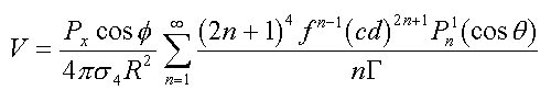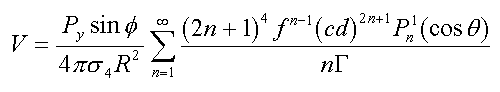
For a Py dipole located along the radial projection at distance f from the center of a sphere

For a Pz dipole located along the radial projection at distance f from the center of a sphere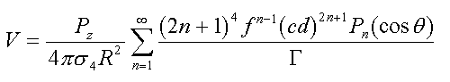

where Pn and {} are Legendre polynomials and for n = 1 to 30 iterations

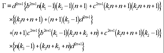
and where

Preparation of this chapter was supported by the National Institute of Mental Health, grants MH30854 and MH40052, and by the Department of Veterans Affairs.

We thank Margaret J. Rosenbloom for her critical comments.

published 2000